
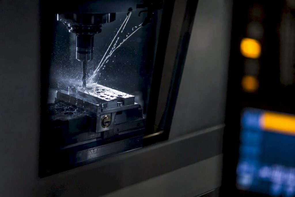
The best practical approach for production CNC is controller-available telemetry, spindle current, power, and axis tags, fused on an edge-enabled digital twin that outputs remaining useful life (RUL) with uncertainty bands. That single change cuts scrapped parts, stretches tool life, and turns replacement from a guess into a scheduled event. The rest of this guide covers the signals worth capturing, the modelling choices that actually work, and the commissioning steps to get there.
TL;DR:
Controller telemetry, such as spindle current and axis tags, can be used for cost-effective, real-time tool wear detection with typical sampling rates between 10 and 50 Hz.
External sensors like vibration and force measurement improve sensitivity, especially for detecting early-stage chipping or crater wear, but come with higher setup and maintenance costs.
Hybrid approaches that combine controller data for every machine with vibration sensors on high-value spindles provide the best balance of cost and accuracy.
Models that fuse multi-signal data through a state-space approach with Kalman filtering have demonstrated reduced RUL prediction errors and high fault detection accuracy.
Implementing robust decision thresholds, alarm integration, and logging at machine and workflow levels is essential for translating predictions into effective maintenance actions.
Table of Contents
-
Should you use controller data or external sensors for tool monitoring?
-
Which predictive model actually works for remaining useful life?
-
What integration challenges come with different CNC machine brands?
-
Preventive vs predictive maintenance after monitoring goes live
What is tool life monitoring in CNC and why does it matter?
Tool life monitoring is the practice of tracking a cutting tool’s condition in real time rather than relying on a fixed cycle count, so you replace it when it’s actually worn, not when a spreadsheet says it should be. The standard industry term for the broader discipline is condition-based maintenance, and it sits alongside adaptive control as one of the two big levers for getting more out of every insert and endmill.
Every cutting tool degrades through a handful of recognisable failure modes. Flank wear is the gradual, predictable erosion along the tool’s relief face and the one most monitoring systems are built to catch. Crater wear forms on the rake face from chip friction and heat, and it’s sneakier because it can weaken an edge without changing the part dimensions much until it’s too late. Chipping and fracture are the sudden failures: a hard inclusion in the stock, a moment of chatter, or a coolant interruption, and the edge is gone in one pass.
The problem with fixed cycle counters is that they treat every job as identical. A tool cutting soft aluminium at a conservative feed will outlast its rated cycle count by a wide margin; the same tool in a harder alloy or an aggressive finishing pass might fail well before the counter says to swap it. That mismatch shows up in three numbers manufacturing engineers actually care about:
-
First-pass yield — how many parts come off the machine within spec without rework.
-
Scrap rate — parts lost to tool failure mid-cut, often the most expensive kind of scrap because it damages fixtures or the workpiece too.
-
Tool-cost per part — the real economic figure once you account for both premature swaps and late, failure-driven ones.
Condition monitoring replaces the guess with a measurement, and that’s the whole point of moving beyond a counter on the control panel.
What signals correlate with CNC tool wear?
Spindle current and power are the most practical starting point because most CNC controllers already expose them, and no extra hardware installation is required. Current draw rises as a worn edge fights the cut, and a control sampling at even 10 to 50 Hz can pick up the trend clearly enough for wear estimation. Some controllers support far higher rates: FANUC-based systems can stream data at up to 1 kHz without bolting on a single sensor, which is enough resolution for genuine anomaly detection rather than just a coarse trend line.
Vibration is the next most useful signal, captured with tri-axial accelerometers mounted near the spindle or workholding. It’s particularly good at catching chatter and the sharp spike that comes with chipping, patterns that spindle current alone can miss because the load change is momentary. Cutting-force measurement, using a dynamometer under the workpiece or in the toolholder, gives the cleanest wear signal of all, but it’s also the most expensive and fiddly to calibrate, which is why it tends to stay in R&D cells rather than production floors.
Round out the picture with:
-
Temperature at the cutting zone or spindle housing, useful for slower-developing wear trends.
-
Acoustic emission sensors, sensitive to the high-frequency signature of crater wear and micro-fracturing.
-
Controller tags — feed rate, spindle speed, tool ID, and axis loads — that give the context needed to interpret every other signal correctly.
Statistic to note: a validated diagnostic rule using a spindle current ratio of roughly one and a half times the baseline load correlated with flank wear exceeding typical ISO wear limits (https://www.mdpi.com/2504-4494/8/5/194), and the same model predicted surface roughness with about 10% average error using current alone.
If you’re retrofitting an older machine, controller tags and spindle current are usually available without touching the machine’s wiring. Vibration and force sensors mean physical installation, which is fine for a new production cell but a harder sell on a fleet of ageing machines.
Should you use controller data or external sensors for tool monitoring?
The controller-data route is the fastest to deploy and the cheapest to scale across a fleet, because you’re reading tags the machine already generates rather than adding hardware to every spindle. Its limit is sensitivity: current and power react well to gradual flank wear but can miss subtle chipping or early-stage crater wear that hasn’t yet loaded the spindle enough to show up.
External sensor stacks, accelerometers, dynamometers, acoustic emission pickups, close that sensitivity gap. The cost is real: calibration per tool and material combination, cabling or wireless telemetry, and ongoing sensor maintenance that a pure software approach doesn’t need.
Most production shops land on a hybrid: controller data as the baseline for every machine, with vibration sensors added selectively on high-value spindles or operations with a history of chipping. The decision usually comes down to three questions:
-
How many machines need coverage, and does the budget stretch to sensors on all of them?
-
Is your critical failure mode gradual (current suffices) or sudden (you need vibration)?
-
Can your network handle the added data volume from tri-axial accelerometers running continuously?
Edge processing matters more than most engineers expect going in. A digital-twin model needs a stable, low-latency read on the machine’s current state, and running that model in the cloud introduces round-trip delays that undermine tight decision loops. Testbed work on fused sensor models has kept the full pipeline, from raw signal to RUL estimate, under a 100-millisecond budget using edge GPU hardware and compact models. That’s fast enough to gate the next cut if the model flags a problem.
Sampling frequency and telemetry alignment are where a lot of pilots quietly fail. If vibration comes in at 10 kHz and spindle power at 20 Hz, fusing them without careful timestamp correction produces a noisy, unstable wear trajectory that no model can forecast reliably. Clock synchronisation isn’t an afterthought here; it’s the foundation the whole predictive layer sits on.
Which predictive model actually works for remaining useful life?
The models that hold up in production don’t try to map raw current or vibration straight to a wear number in micrometres. They build a latent “wear index,” a dimensionless internal state derived from fused signals, and forecast that instead. A state-space model with Kalman filtering is what stabilises this latent trajectory against sensor noise and the natural variability of a real production floor.
On top of that state-space core, two model families do the heavy lifting for RUL prediction:
-
LSTM networks — compact enough to run on edge hardware, well suited to the sequential nature of wear progression, and the default choice for shop-floor deployment.
-
Small Transformer models — higher accuracy in exchange for more compute, worth considering when a single edge box is already serving several spindles.
Neither model type should hand an operator a single number and call it done. Uncertainty-aware outputs, using techniques like Monte Carlo dropout to generate a confidence band around the prediction, are what let you build sensible decision rules: defer the swap if confidence is high and RUL is comfortably ahead of the next job, alarm if confidence drops sharply, schedule a change during the next natural pause if the trend is clear but not urgent.
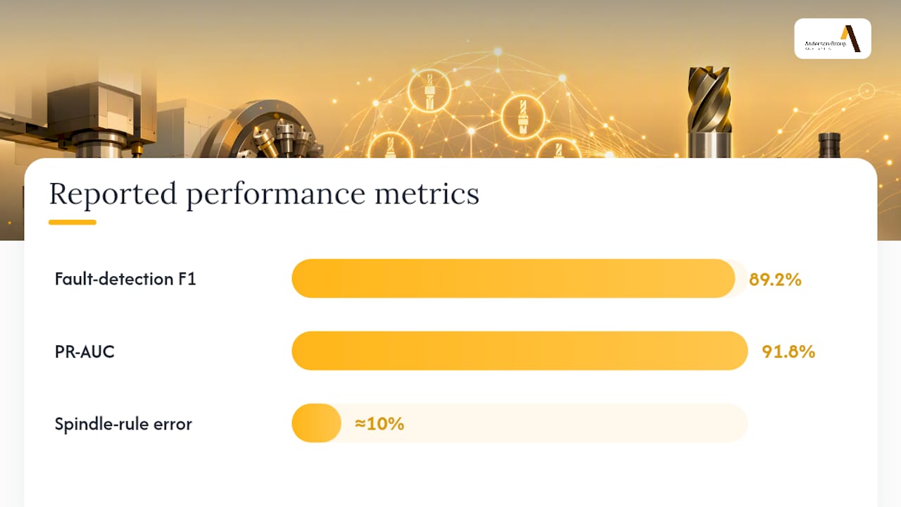
The performance numbers back the approach up. Fusing multi-rate vibration, spindle current, and temperature through a state-space core with Kalman filtering reduced RUL prediction error (RMSE) by a clear margin(https://www.mdpi.com/2075-1702/14/3/335) on a CNC testbed, with fault-detection F1 climbing to around 0.892 and PR-AUC to 0.918. Separately, a digital-twin framework using LSTM achieved flank-wear prediction with low RMSE in controlled testing(https://link.springer.com/article/10.1007/s10845-025-02606-4) in controlled testing, with real-time deployment validated at a higher but still workable error margin.
| Modelling approach | Typical use case | Reported performance |
|---|---|---|
| State-space + Kalman filter | Stabilising noisy multi-signal fusion | RUL prediction error reduced by a clear margin |
| LSTM digital twin | Edge-deployed flank wear prediction | low RMSE in controlled testing |
| Spindle-current threshold rule | Low-cost, non-intrusive wear flag | ~10% average error on surface roughness prediction |
These aren’t lab curiosities. They’re the kind of number you can hold a vendor or an internal pilot to when you’re deciding whether a model is ready for the shop floor.
How should predictions trigger action on the machine?
A prediction is only useful if it changes what happens next, and the decision rule that connects RUL output to actual machine behaviour needs to be designed before the model goes live, not bolted on afterwards.
-
Set confidence-weighted thresholds. High confidence and comfortable RUL means run to the next scheduled stop. High confidence and low RUL means alarm now. Low confidence, regardless of the point estimate, means flag for manual inspection rather than trusting the number blindly.
-
Wire the alarm into the HMI, not just a dashboard. Operators respond to what’s in front of them on the machine, not a report they check once a shift.
-
Where the control supports it, gate the next cut automatically rather than just alarming, particularly for lights-out runs where nobody is on the floor to react.
-
Feed the same fields into your maintenance workflow or MES: tool ID, predicted RUL at time of change, actual wear observed, and job context. That record is what lets you validate and retrain the model instead of running it blind indefinitely.
-
Close the loop with adaptive feed control where the toolpath allows it. Adaptive strategies that adjust feed dynamically based on predicted cutting load have shown production time cut by up to 12.8% and tool life extended by up to 41.7% in experimental comparisons, well beyond what a static, alarm-only setup delivers.
Pro Tip: Log every actual tool change, even the ones triggered manually rather than by the model, against the RUL prediction that was live at the time. That comparison is the fastest way to catch a model that’s quietly drifting before it causes a scrap run.
How do you commission a tool life monitoring system?
Getting from a spreadsheet-based tool counter to a working predictive system is a sequence, not a single install, and skipping steps here is where most pilots stall.
-
Confirm controller access first. Check whether your machine exposes OPC UA, MTConnect, or FOCAS, and run a baseline capture before changing anything so you have a clean reference signal.
-
Synchronise clocks across every data source. Multi-rate fusion falls apart without deterministic, timestamped windows, which is why NTP or PTP correction belongs at the top of the checklist, not the bottom.
-
Choose your signal set and sampling windows deliberately, matching resolution to the failure mode you’re actually trying to catch rather than defaulting to “capture everything.”
-
Bootstrap the model with labelled wear data, either from periodic vision inspection on the floor or controlled lab runs where wear is measured directly against the signals.
-
Set commissioning acceptance criteria before go-live, not after. A reasonable early target sits near the RMSE and F1 figures validated in testbed research, with a latency budget under 100 milliseconds for edge-deployed models.
-
Plan for drift from day one. Rehearsal-based continual learning, retraining periodically on recent buffered windows plus a small rehearsal set of older data, keeps the model accurate as tool geometry, material batches, or cutting strategy change over time.
Treat the first machine as a pilot, not a rollout. Practitioner guidance consistently points toward validating on one cell before scaling the same model architecture across similar machines.
Assessing monitoring requirements when selecting machinery
Before planning tool-life monitoring, identify the controller signals, interfaces and permissions available on the exact machine. Confirm that the proposed monitoring system can use those data.
Agree who will verify controller connectivity and data availability before approving a monitoring pilot. Confirm any machinery-supplier and integration work separately.
For teams evaluating whether a monitoring pilot is worth the investment, the KPIs worth tracking post-deployment are consistent across most deployments:
-
Uptime improvement, measured against your current unplanned-stoppage rate.
-
Scrap reduction, specifically scrap tied to tool failure rather than general process variation.
-
Tool-cost per part, the single number that captures whether the whole exercise paid for itself.
Types of CNC tools and their specific wear patterns
Different tool types wear in genuinely different ways, and a monitoring system tuned for one can miss failures in another entirely. End mills, especially in aluminium or steel roughing, tend toward gradual flank wear on the peripheral cutting edges, which is exactly the slow, current-detectable trend that spindle-power monitoring handles well.
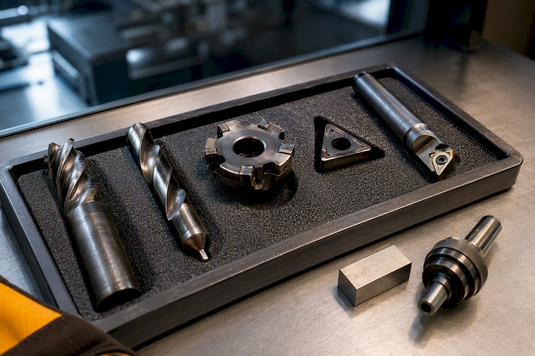
Drills behave differently: wear concentrates at the margin and the point, and a drill nearing failure often shows a sharper thrust-force spike rather than a smooth current climb, which is why some shops add vibration sensing specifically on drilling operations. Face mills, running multiple inserts simultaneously, complicate monitoring further because a single worn insert among six or eight healthy ones can hide inside an averaged current signal.
Inserts used in turning show classic crater wear on the rake face from continuous chip contact, a mode that’s harder to catch with current alone because crater wear can progress well before it affects cutting load significantly. Taps and threading tools fail more abruptly, often through fracture from chip packing or misalignment, which pushes them toward acoustic emission or vibration monitoring rather than a slow-trend current model.
Composite and advanced-material cutters, increasingly common in aerospace work, wear through abrasive mechanisms that don’t map neatly onto the flank/crater framework built for metals, and monitoring these often needs a materials-specific baseline rather than a generic threshold. The practical takeaway: match your signal choice and your alarm thresholds to the tool type and material in front of you, not a single blanket rule across the whole shop.
What integration challenges come with different CNC machine brands?
Every controller brand exposes its data differently, and that’s the single biggest practical obstacle to scaling a monitoring system across a mixed fleet. FANUC controls, common across a huge share of installed machines, support FOCAS for programmatic access and can stream at high frequency, but the protocol and available tag list differ from what you’ll find on a Siemens or Heidenhain control.
Older machines are the harder case. A control from a decade or more ago may expose almost nothing beyond basic status bits, forcing a choice between a controller retrofit, an external sensor package, or accepting a coarser monitoring approach on that machine while newer units in the fleet get the full treatment. Mixed-brand shops often end up running two or three different data-collection methods simultaneously, which complicates the fusion layer that’s supposed to combine everything into one consistent wear index.
MTConnect has become a common bridging standard precisely because it normalises data across brands into a shared format, reducing the integration burden of writing brand-specific connectors for every machine on the floor. Even so, tag naming, sampling rate limits, and what’s actually exposed at the controller level vary enough that a “collect everything from every machine the same way” plan rarely survives first contact with a real fleet.
The practical fix is sequencing: standardise on the newest, most capable machines first, prove the model architecture works, then build brand-specific adapters for older or less transparent controls rather than trying to solve every integration problem before the first pilot runs.
Preventive vs predictive maintenance after monitoring goes live
Preventive maintenance, changing tools on a fixed schedule regardless of actual condition, doesn’t disappear once a monitoring system is running. It shifts role: instead of being the primary replacement trigger, it becomes the safety net for tools that aren’t yet instrumented or for failure modes the model hasn’t been trained to catch.
Predictive maintenance, driven by the RUL model, becomes the primary policy for anything the monitoring system covers well. The shift changes how a maintenance team plans its week: instead of a fixed swap list generated from cycle counts, the schedule now responds to what the model is actually forecasting, which usually means fewer total swaps but better-timed ones.
The transition isn’t instant and shouldn’t be treated as a light switch. Running both systems in parallel for a defined period, comparing predicted RUL against a preventive schedule’s fixed intervals, is how you build confidence the model is actually more accurate than the counter it’s replacing. Once that comparison consistently favours the model, the preventive schedule can be relaxed for that tool and operation, while remaining as a fallback for sensor outages or unexpected controller downtime.
The other change worth planning for is skills, not just process. Maintenance teams accustomed to reading a wear-out schedule need to get comfortable interpreting a confidence band and a defer/alarm/schedule recommendation instead, and that’s a training investment as real as the sensor installation itself.
Is tool life monitoring worth the investment?
The upfront cost of a monitoring system varies enormously depending on the approach: a controller-data-only setup on machines with accessible telemetry costs little beyond integration engineering time, while a full sensor stack with vibration, force, and acoustic emission monitoring across a fleet represents a genuine capital investment plus ongoing calibration.
The return shows up in three places that are each individually measurable. Reduced scrap from mid-cut tool failures is usually the fastest payback, because a single scrapped aerospace-grade billet or a damaged fixture can outweigh months of monitoring system cost on its own. Extended tool life from condition-based rather than schedule-based replacement compounds over a fleet, particularly for expensive tooling used across high-value materials. Reduced unplanned downtime from catching a failing tool before it breaks mid-cycle protects the production schedule itself, not just the part.
The honest caveat is that the payback period depends heavily on your current baseline. A shop already running tight preventive schedules with low scrap will see a smaller relative gain than one currently running tools to failure on a fixed counter with no condition feedback at all. Before committing capital, it’s worth quantifying your current tool-cost per part and scrap rate tied specifically to tool failure, because that baseline is what determines whether a sensor stack pays for itself in months or years.
For shops evaluating a phased approach, starting with controller-data monitoring on the highest-value or highest-failure-rate machines gives a real-world payback estimate before extending to a full sensor deployment, a far lower-risk path than committing to fleet-wide sensor hardware on day one.
Author perspective: where tool-life monitoring is heading
Digital twins and edge fusion matter because they scale in a way single-sensor thresholds never will. A current-ratio rule works brilliantly on one machine cutting one material; it breaks the moment your job mix changes, which is most shops, most weeks.
The caveat I’d stress hardest: don’t let one strong signal make you overconfident. The RMSE and F1 figures in this piece came from fused models, not single sensors, and that fusion is doing real work.
My recommendation is unglamorous but reliable: pilot on one machine, measure the actual ROI against your current scrap and downtime numbers, then scale with rehearsal-based updates rather than a one-off training run you never revisit.
How Anderson supports a monitoring-ready production line
Discuss controller interfaces and available options when comparing machinery. Data access varies by controller, licensing and configuration, so verify it before selecting a monitoring approach.

Contact Anderson Australia about the proposed machine configuration and available controller interfaces. Confirm monitoring software, integration and specialist support with the responsible providers, and include their scope in the pilot plan.
Sources
-
Intelligent real-time tool life prediction for a digital twin framework
-
Development of a method and a smart system for tool critical life real-time monitoring